---
slug: "statspai"
source_type: "readme"
source_url: "https://cdn.jsdelivr.net/gh/brycewang-stanford/StatsPAI@main/README.md"
repo: "https://github.com/brycewang-stanford/StatsPAI"
source_file: "README.md"
branch: "main"
---
[English](https://github.com/brycewang-stanford/statspai/blob/main/README.md) | [中文](https://github.com/brycewang-stanford/statspai/blob/main/README_CN.md)
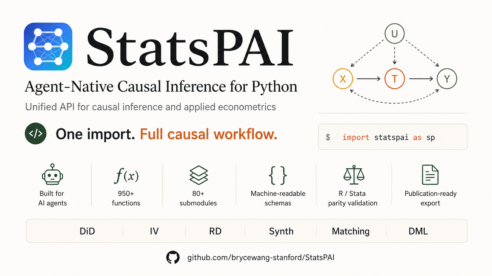
# StatsPAI: an Agent&Python-native Stata/R replacement for applied causal inference
[](https://pypi.org/project/StatsPAI/)
[](https://pypi.org/project/StatsPAI/)
[](https://github.com/brycewang-stanford/statspai/blob/main/LICENSE)
[](https://github.com/brycewang-stanford/statspai/actions)
[](https://brycewang-stanford.github.io/StatsPAI/)
[](https://pepy.tech/projects/statspai)
[](https://joss.theoj.org/papers/9f1c837b1b1df7adfcdd538c3698e332)
[](https://doi.org/10.5281/zenodo.19933900)
StatsPAI is for empirical researchers who would normally jump between Stata, R,
and Python. Its goal is to make common Stata/R econometrics and causal-inference
workflows feel native in Python: load a dataset, estimate a model, inspect
diagnostics, export tables, and hand the result to an agent or notebook without
leaving one API.
It is meant to be a practical replacement path for new Python-first work:
- Stata-style routines: `regress`, `ivregress`, `reghdfe`, `csdid`, `rdrobust`,
`synth`, `psmatch2`, `outreg2`.
- R-style routines: `lm`, `fixest`, `did`, `rdrobust`, `Synth`, `DoubleML`,
`MatchIt`, `modelsummary`, `broom`.
- Python-native outputs: `.summary()`, `.tidy()`, `.plot()`, `.to_latex()`,
`.to_docx()`, `.to_agent_summary()` where supported by the result object.
- Companion Stata tooling: our own
[`stata-code`](https://github.com/brycewang-stanford/stata-code/) can work
with StatsPAI so agents can understand existing Stata workflows, translate
them into Python, and cross-check results more smoothly.
- Companion skill repos:
[`Auto-Empirical-Research-Skills`](https://github.com/brycewang-stanford/Auto-Empirical-Research-Skills),
[`AER-Skills`](https://github.com/brycewang-stanford/AER-Skills),
[`Awesome-Journal-Skills`](https://github.com/brycewang-stanford/Awesome-Journal-Skills),
and [`Paper-WorkFlow`](https://github.com/brycewang-stanford/Paper-WorkFlow)
can work alongside StatsPAI and an agent as the methods, journal, manuscript,
and reproducibility skill layer.
StatsPAI is not a promise that every Stata/R command is bit-for-bit identical.
When exact external parity matters, use the `validation_status` metadata,
the reference-parity tests, and `sp.cross_validate` to see what has been
certified for that estimator. `validation_status` distinguishes
certified/validated evidence from API-stable breadth: a `certified` or
`validated` symbol carries numerical evidence, while `api_stable` denotes a
stable interface without a numerical-parity claim.
---
## Install
```bash
pip install statspai
```
Then:
```python
import statspai as sp
print(sp.datasets.list_datasets()[["name", "design", "n_obs"]].head())
```
StatsPAI ships teaching datasets such as Card (1995), Callaway-Sant'Anna
`mpdta`, Lee (2008) RD, LaLonde/NSW, and California Proposition 99. The examples
below run offline after installation.
At a glance: 1,147 registered functions across 87 submodules; 352k LOC (core) + 200k LOC (tests). Run `python scripts/registry_stats.py` to reproduce these numbers.
---
## If You Come From Stata Or R
| What you used before | Stata / R examples | StatsPAI entry point |
| --- | --- | --- |
| OLS / robust SE | `reg y x, vce(robust)` / `lm()` + `sandwich` | `sp.regress(..., robust="hc1")` |
| IV / 2SLS | `ivregress 2sls` / `AER::ivreg()` | `sp.ivreg("y ~ (d ~ z) + x", data=df)` |
| High-dimensional FE | `reghdfe` / `fixest::feols()` | `sp.feols("y ~ x | firm + year", data=df)` |
| Staggered DiD | `csdid` / `did::att_gt()` | `sp.callaway_santanna()` + `sp.aggte()` |
| Regression discontinuity | `rdrobust` / `rdrobust::rdrobust()` | `sp.rdrobust()` |
| Synthetic control | `synth` / `Synth::synth()` | `sp.synth()` |
| Matching / PSM | `psmatch2` / `MatchIt` | `sp.psmatch2()` and matching helpers |
| Publication tables | `outreg2`, `esttab` / `modelsummary` | `sp.outreg2()`, `sp.modelsummary()` |
---
## Compared With Other Python Causal Packages
StatsPAI is meant to be the broad Stata/R-style workbench for applied empirical
research, not only a single modeling family.
| Package | Best fit | Where StatsPAI is different |
| --- | --- | --- |
| [`causallib`](https://github.com/BiomedSciAI/causallib) | Observational causal inference with a scikit-learn-style workflow: IPW, matching, standardization, doubly robust estimation, and evaluation. | StatsPAI is broader for Stata/R migration: OLS, IV, high-dimensional FE, DiD, RD, synthetic control, matching, diagnostics, validation metadata, and publication-table export in one API. |
| [`CausalPy`](https://github.com/pymc-labs/CausalPy) | Bayesian causal analysis for quasi-experimental settings, built around PyMC models, uncertainty, and visual diagnostics. | StatsPAI prioritizes familiar Stata/R econometrics commands, frequentist workflows, cross-language parity evidence, bundled teaching datasets, and agent-ready result summaries. |
Use `causallib` when you mainly want sklearn-style treatment-effect pipelines.
Use `CausalPy` when you want Bayesian causal modeling in PyMC. Use StatsPAI when
you want one Python package to replace the everyday Stata/R empirical workflow.
---
## Beginner Examples With Results
The outputs below are rounded from the bundled examples in this repository
using StatsPAI 1.20.0.
### 1. OLS: the first `regress` / `lm` replacement
Question: how much higher is log wage for one more year of schooling in the
Card (1995) teaching dataset?
```python
import statspai as sp
card = sp.datasets.card_1995()
ols = sp.regress(
"lwage ~ educ + exper + expersq + black + south + smsa",
data=card,
robust="hc1",
)
print(ols.summary())
```
Result:
```text
Model: OLS
Dependent Variable: lwage
Coefficient Std. Error t-statistic P>|t|
Intercept 4.8388 0.0637 76.0131 0.0000
educ 0.1100 0.0041 26.5543 0.0000
exper 0.0283 0.0054 5.2742 0.0000
expersq -0.0005 0.0002 -2.2132 0.0270
black -0.1561 0.0231 -6.7571 0.0000
south -0.0554 0.0193 -2.8636 0.0042
smsa 0.0905 0.0205 4.4214 0.0000
R-squared: 0.2307
```
Read it like a Stata/R regression table: in this replica, one additional year
of schooling is associated with about `0.110` higher log wage, before dealing
with endogeneity. Adding the standard Card (1995) controls (experience and
its square, race, region, SMSA) lifts R² from `0.210` to `0.231` and the
educ coefficient is essentially unchanged — the small attenuation from
classical measurement error in `educ` persists and motivates the IV in
example 2.
### 2. IV / 2SLS: replace `ivregress 2sls` or `AER::ivreg`
Question: instrument education with proximity to a four-year college (`nearc4`).
```python
import statspai as sp
card = sp.datasets.card_1995()
iv = sp.ivreg(
"lwage ~ (educ ~ nearc4) + exper + expersq + black + south + smsa",
data=card,
)
print(iv.summary())
```
Result:
```text
Model: IV-2SLS
Dependent Variable: lwage
Coefficient Std. Error t-statistic P>|t|
educ 0.1418 0.0188 7.5606 0.0000
Model Diagnostics:
First-stage F (educ): 159.8305
Partial R2 (educ) : 0.0505
Hausman p-value : 0.0322
```
StatsPAI prints the coefficient and the diagnostics you would usually collect
with separate post-estimation calls.
### 3. Staggered DiD: replace `csdid` or R `did`
Question: what is the average minimum-wage effect on teen employment in the
Callaway-Sant'Anna `mpdta` example?
```python
import statspai as sp
mp = sp.datasets.mpdta()
gt = sp.callaway_santanna(
data=mp,
y="lemp",
t="year",
i="countyreal",
g="first_treat",
)
overall = sp.aggte(gt, type="simple", bstrap=False)
print(overall.summary())
```
Result:
```text
Callaway and Sant'Anna (2021) - aggte[simple]
ATT: -0.032977
Std. Error: 0.005493
95% CI: [-0.043742, -0.022211]
P-value: 0.0000
Observations: 2,500
```
The headline estimate is negative and statistically precise in this bundled
replica.
### 4. Regression discontinuity: replace `rdrobust`
Question: is there an incumbent advantage at the zero-margin cutoff in the Lee
(2008) Senate election design?
```python
import statspai as sp
lee = sp.datasets.lee_2008_senate()
rd = sp.rdrobust(data=lee, y="voteshare_next", x="margin", c=0)
print(rd.summary())
```
Result:
```text
Sharp RD Estimation
RD Effect: 0.061599
Std. Error: 0.022662
95% CI: [0.017183, 0.106015]
P-value: 0.0066
Bandwidth H: 0.042287
N Effective Left: 440
N Effective Right: 443
```
The robust bias-corrected RD estimate is about `0.062` vote-share points.
### 5. Synthetic control: replace Stata/R `synth`
Question: how did California's Proposition 99 affect cigarette sales?
```python
import statspai as sp
prop99 = sp.datasets.california_prop99()
sc = sp.synth(
data=prop99,
outcome="cigsale",
unit="state",
time="year",
treated_unit="California",
treatment_time=1989,
)
print(sc.summary())
```
Result:
```text
Synthetic Control Method
ATT: -13.085166
Std. Error: 4.164718
95% CI: [-21.247862, -4.922469]
P-value: 0.0789
Active donor weights:
Montana 0.8420
Nevada 0.1580
```
The estimate says California consumed about 13 fewer packs per capita after
the intervention in this replica.
---
## Export Results
Every result object ships with `Stata`-style and `R` (modelsummary/broom)
exporters. One call drops a multi-sheet `.xlsx` or a Word table that you can
hand to a co-author.
```python
sp.outreg2(r1, r2, filename="results.xlsx") # Excel, Stata-style
sp.modelsummary(r1, r2, output="table.docx") # Word, modelsummary-style
```
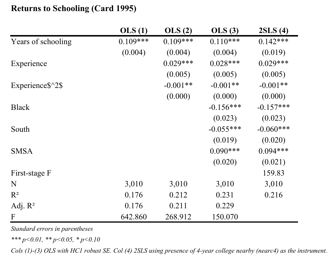
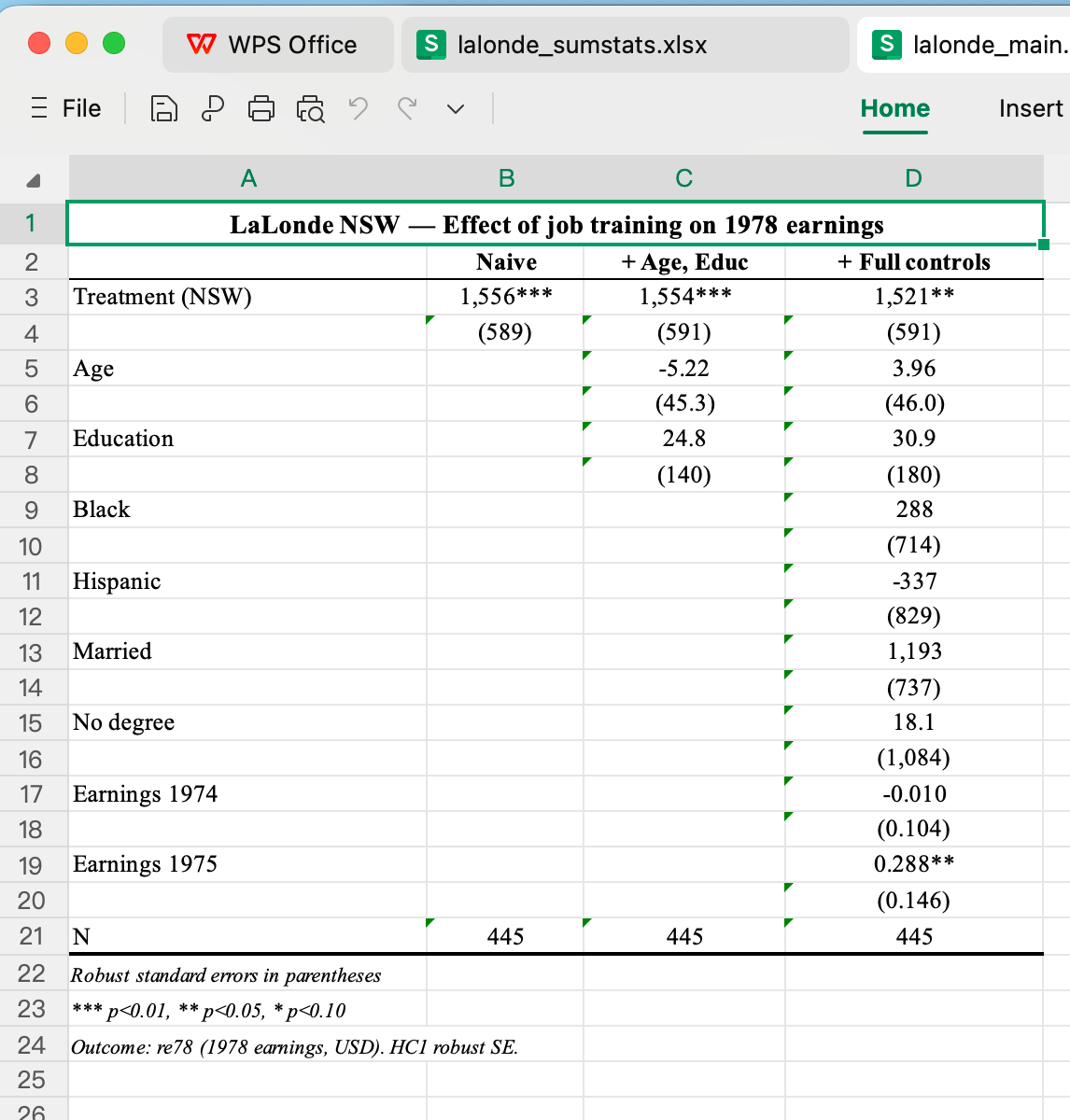
The screenshots above are the `.xlsx` output of `sp.outreg2` on the Card (1995)
OLS + IV pair and the LaLonde/NSW propensity-score regression. Each sheet
contains the coefficient table, model-fit statistics, and significance stars
in the format your journal template expects.
---
## Interactive Plot Editing
If you miss Stata's Graph Editor, use `sp.interactive(fig)` on any matplotlib
figure returned by StatsPAI. It opens a Jupyter editing panel with a live
preview, so beginners can adjust a figure without learning every matplotlib
option first.
What it is for:
- change titles, labels, fonts, colors, markers, line widths, grids, legends,
axis limits, figure size, and export DPI;
- switch among publication-oriented themes, including academic, ggplot-like,
FiveThirtyEight-style, and dark presentation styles;
- keep the data layer protected while editing cosmetic elements;
- export reproducible Python code for the edits, so the final figure can be
regenerated from a script instead of being only a manual screenshot.
```python
import statspai as sp
mp = sp.datasets.mpdta()
gt = sp.callaway_santanna(data=mp, y="lemp", t="year",
i="countyreal", g="first_treat")
agg = sp.aggte(gt, type="dynamic", bstrap=False)
fig, ax = sp.ggdid(agg)
editor = sp.interactive(fig) # edit the plot in Jupyter
print(editor.generate_code()) # copy reproducible matplotlib edits
```
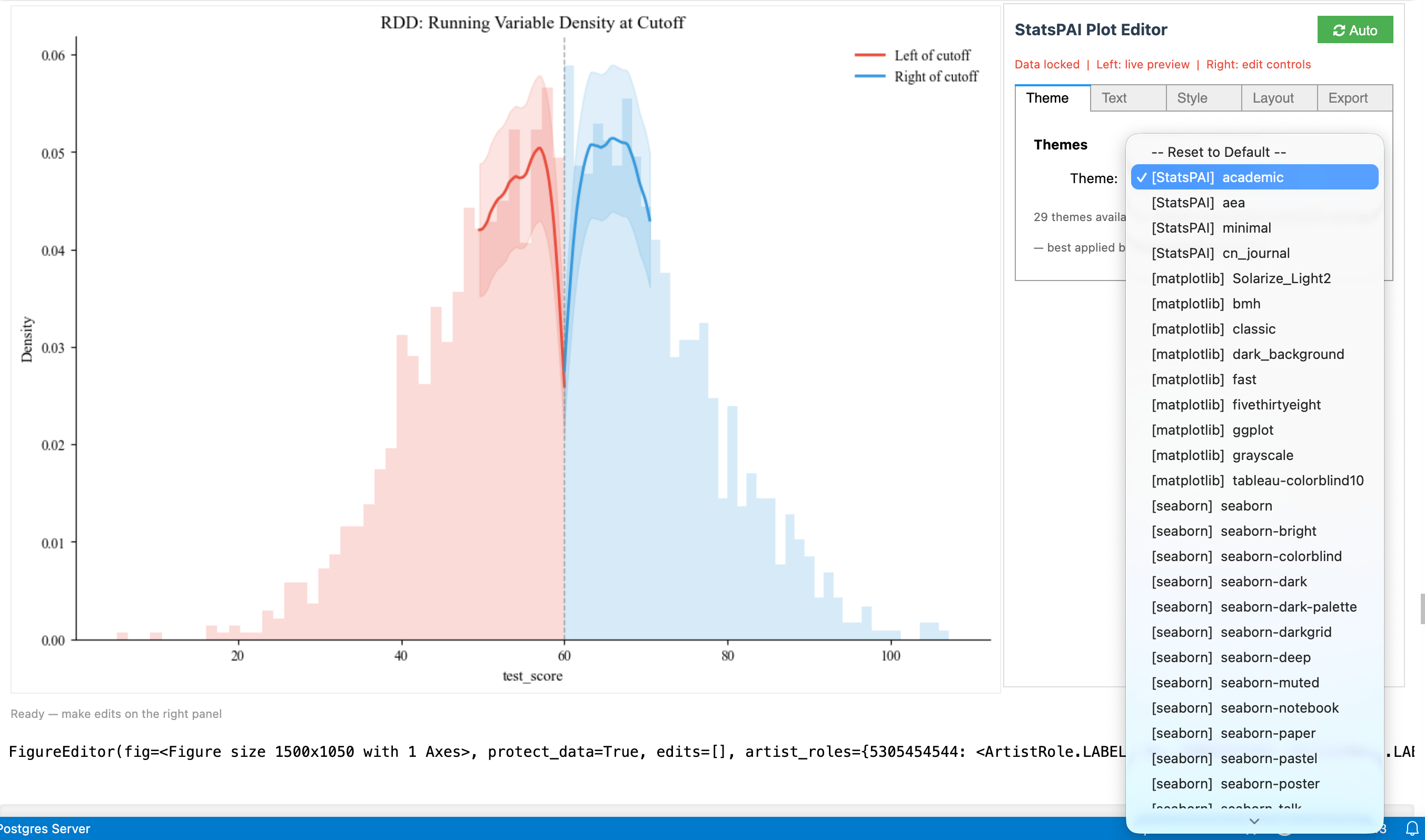
The screenshot above shows the intended workflow: preview on one side, editing
controls on the other, and code export for reproducibility.
---
## Everyday Workflow
```python
import statspai as sp
card = sp.datasets.card_1995()
r1 = sp.regress(
"lwage ~ educ + exper + expersq + black + south + smsa",
data=card,
robust="hc1",
)
r2 = sp.ivreg("lwage ~ (educ ~ nearc4) + exper + expersq + black + south + smsa", data=card)
print(r1.summary()) # human-readable table
print(r1.tidy().head()) # broom-style dataframe
sp.modelsummary(r1, r2, output="table.docx") # Word table
sp.outreg2(r1, r2, filename="results.xlsx") # Stata-style export
```
Useful docs:
- [Getting started](https://github.com/brycewang-stanford/StatsPAI/blob/HEAD/docs/getting-started.md)
- [Cookbook](https://github.com/brycewang-stanford/StatsPAI/blob/HEAD/docs/cookbook.md)
- [Choosing an IV estimator](https://github.com/brycewang-stanford/StatsPAI/blob/HEAD/docs/guides/choosing_iv_estimator.md)
- [Choosing a DID estimator](https://github.com/brycewang-stanford/StatsPAI/blob/HEAD/docs/guides/choosing_did_estimator.md)
- [Choosing an RD estimator](https://github.com/brycewang-stanford/StatsPAI/blob/HEAD/docs/guides/choosing_rd_estimator.md)
- [Migrating from R to StatsPAI](https://github.com/brycewang-stanford/StatsPAI/blob/HEAD/docs/guides/migration-from-r.md)
- [Exporting regression tables](https://github.com/brycewang-stanford/StatsPAI/blob/HEAD/docs/guides/exporting-regression-tables.md)
---
## Validation And Agent Use
StatsPAI has a large API surface, so validation status matters.
```python
import statspai as sp
print(sp.describe_function("ivreg")["validation_status"])
print(sp.list_functions(validation_status="certified")[:5])
```
Use the validation metadata to distinguish:
- certified functions with external numerical evidence;
- validated functions with internal or published-reference checks;
- API-stable functions whose interface is stable but whose exact Stata/R parity
may be design-dependent;
- experimental functions for frontier workflows.
Agent-facing metadata is available through `sp.list_functions()`,
`sp.describe_function()`, and `sp.function_schema()`.
### Cross-language parity, made queryable
The validation tier above has a richer, auditable backing: a **parity index**
where every verified function records *what it was aligned against, to what
tolerance, on which test, and how closely it matched*. Each row traces to a
committed test artifact (the pinned StatsPAI ↔ R ↔ Stata harness, version-locked
via `renv.lock` + per-run provenance) — nothing is asserted from memory.
```python
import statspai as sp
sp.parity_status("feols")
# {'status': 'bit-exact', 'reference': 'fixest::feols',
# 'reference_versions': {'R': '...4.5.2...', 'fixest': '0.14.0'},
# 'tolerance': 'rel_est<=1e-06, rel_se<=1e-06', 'headline': {...}, 'test': [...]}
sp.parity_summary() # honest coverage counts (verified vs unverified)
sp.parity_matrix(status="bit-exact")
```
Grades: `bit-exact` (machine tolerance vs a named R/Stata reference), `aligned`
(documented looser tolerance), `analytical-only` (recovers a known DGP truth),
`external-replication` (published-paper numbers), and `unverified` (registered
but no parity evidence attached **yet** — the honest gap). The full,
auto-generated matrix is published at
[docs/parity.md](https://brycewang-stanford.github.io/StatsPAI/parity/).
Beyond point-parity, a Track-B coverage study runs `B=1000` Monte Carlo
replications per estimator and checks that 95% confidence intervals hit their
nominal rate on known-truth DGPs. The seven materialized nominal rows — OLS on
an RCT (0.952), a 2×2 DiD (0.955), strong-instrument IV (0.962),
Callaway–Sant'Anna staggered ATT (0.946), entropy balancing (1.000), DML IRM
ATE (0.969), and a causal-forest AIPW ATE (0.977) — all land in or above the
acceptance band around nominal 0.95; the committed artifacts live under
`tests/coverage_monte_carlo/results_b1000/`.
---
## Changelog
Release notes live outside the README:
- [CHANGELOG.md](https://github.com/brycewang-stanford/StatsPAI/blob/HEAD/CHANGELOG.md) for the full version history.
- [Docs changelog page](https://brycewang-stanford.github.io/StatsPAI/changelog/)
for the rendered documentation site.
The README is intentionally focused on first-time users.
---
## Reviewers
StatsPAI is under JOSS review. Reviewers can start with:
- [JOSS reviewer guide](https://github.com/brycewang-stanford/StatsPAI/blob/HEAD/docs/joss_reviewer_guide.md)
- [JOSS validation dossier](https://github.com/brycewang-stanford/StatsPAI/blob/HEAD/docs/joss_validation_dossier.md)
- [Design rationale and FAQ](https://github.com/brycewang-stanford/StatsPAI/blob/HEAD/docs/joss_reviewer_qa.md)
- [Examples](https://github.com/brycewang-stanford/StatsPAI/tree/HEAD/examples/)
- [Contributing](https://github.com/brycewang-stanford/StatsPAI/blob/HEAD/CONTRIBUTING.md)
- [Support](https://github.com/brycewang-stanford/StatsPAI/blob/HEAD/SUPPORT.md)
---
## Citation
If you use StatsPAI in research, cite the package and the underlying method
papers for each estimator. `sp.citation()` returns the package citation, and
many result objects expose estimator-level citation helpers.
```bibtex
@software{wang2026statspai,
author = {Wang, Biaoyue and Rozelle, Scott},
title = {StatsPAI: Validation-Tiered Causal Inference and
Econometrics Workflows for Python},
year = {2026},
version = {1.20.0},
url = {https://github.com/brycewang-stanford/StatsPAI}
}
```
---
## License
MIT. See [LICENSE](https://github.com/brycewang-stanford/StatsPAI/tree/HEAD/LICENSE).